Multifractals

Although some of the fractals we have drawn have been in color, the colors have not been part of the fractal structure.

They were added for artistic effect (Voss' and Musgrave's landscapes, for example) or for pedagogical reasons (emphasizing the decomposition into pieces for an IFS or the escape rate for a Julia set).

We could represent all the pictures just as well in black and white: a point is black if it belongs to the fractal, otherwise it is white.

Many natural examples are not so clear-cut.

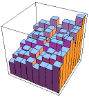
A. As a first mathematical example, we see that by adjusting the probabilities, we can make different parts of the fractal fill in at different rates.

Here is an example. The IFS of this example generates the unit square.

However, the square fills up in a non-uniform way, revealing many fractals.

Here is a review exercise on addresses.

B. Continuing with the example of A., here are histograms representing the probabilities of the first four generations.

Note the highest-probability region has a familiar shape.

This is easy to understand.

The lower left, lower right, and upper right transformations all have the same probability, and those three transformations together generate a Sierpinski gasket.

C. Here is another example, Example B, with p₁ = 0.2, p₂ = p₃ = 0.25, and p₄ = 0.3.

Now structures more complicated than gaskets will appear.

Here is a practice exercise on probabilities, using the probabilities of Example B.

Here is a practice exercise on coarse Holder exponents, using the probabilities of Example B.

D. In the length->0 limit, the coarse Holder exponent becomes a local Holder exponent.

The place-dependence of local Holder exponent motivates the name multifractal.

Here we investigate the distribution of local Holder exponents for Example B.

The resulting curve is called the f(alpha) curve.

Here are some review exercises for the Moran equation.

Here are some practice exercises on moments.

E. Here is the general method for generating multifractals with IFS.

We modify the Moran equation, weighting each term with the probability of the transformation.

This gives the tau(q) curve, from which the f(alpha) curve can be calculated.

Here are some practice exercises for the tau(q) curve.

Here are some practice exercises for the f(alpha) curve.

F. By changing the probabilities of the transformations, we alter the rate at which different parts of the shape fills in, and consequently change the f(alpha) curve.

Here we illustrate this dependence by several examples.

Here we dsicuss the method of moments for plotting f(alpha) curves. This is most easily understood in the context of examples: time series moments, planar data moments, and the special case of IFS moments.

G. Here are some examples of f(alpha) curves derived from financial data using the method of moments.