Exoplanets
I am interested in searching for exoplanets and studying their atmospheres, as a first step towards finding extra-terrestrial life.
We have developed a data-based model-free method that characterizes the data as a multifractal and utilizes the noise
as a source of information. This method then extracts the timescales related to exoplanet's both primary and secondary
transits. These timescales, in combination with simple geometry, can then be used to compute the physical parameters of the
system, which otherwise are the output of model-fitting to data. Being a completely data-driven method, it is free from any
model assumptions and therefore provides a unique and robust framework to detect exoplanets and probe their atmosphere.
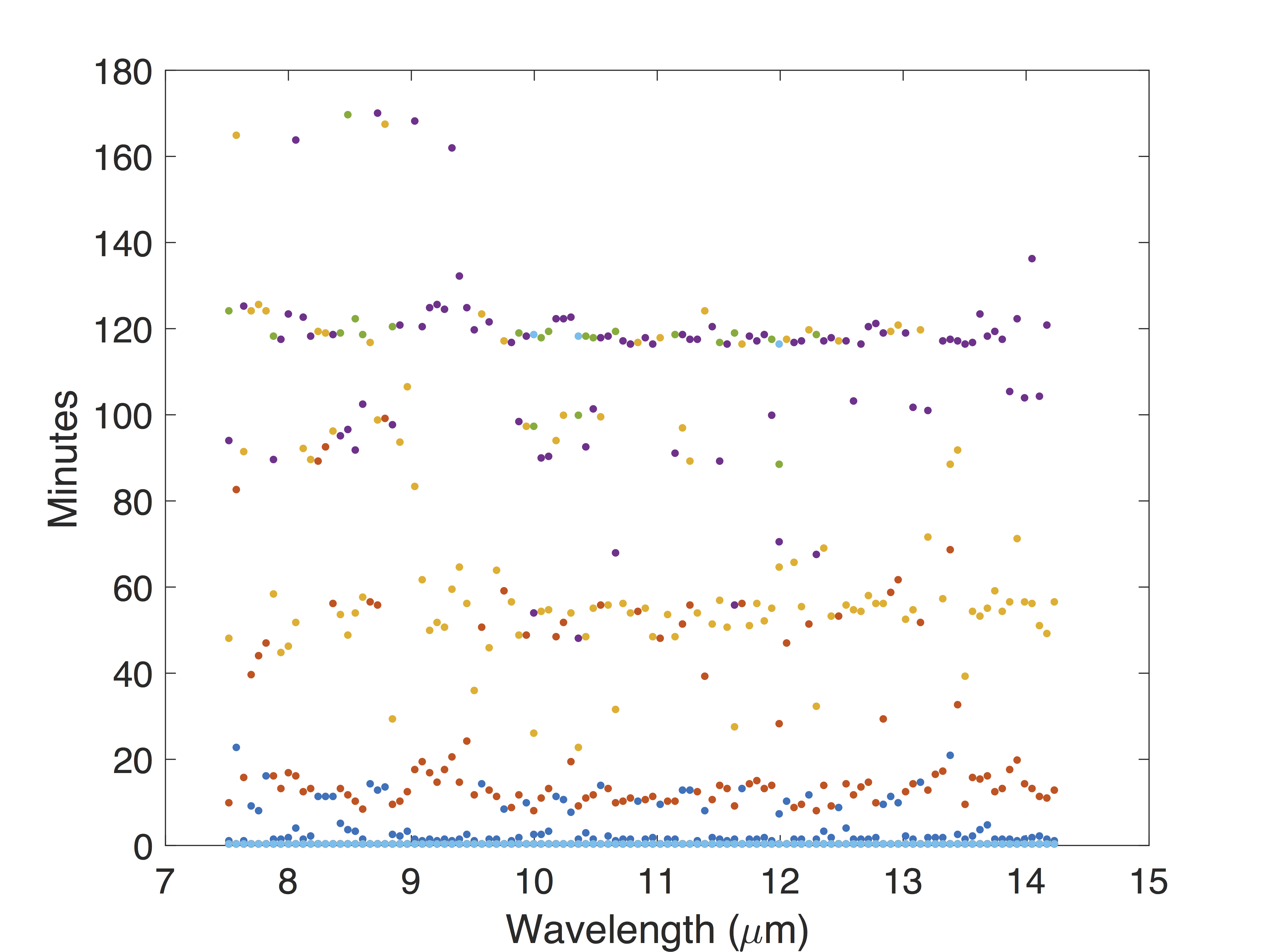
Detection of an exoplanet based on transit timescales.
Reproduced from Figure 5 of Agarwal et al. (2017). Spitzer based crossover times plotted for all wavelengths, for HD 189733b. All four significant timescales (ingress/egress,
full eclipse, complete transit, and Spitzer Wobble timescales), are robustly extracted using our method. These timescales
can then be compute key physical characteristics of the system using simple geometry, rather than fitting parameters of
that geometry.
Probing exoplanet's atmospheres.
Reproduced from Figure 1 of Agarwal et al. (2017). Sampling the planetary limb (terminator) during a secondary eclipse event. While the widely studied emergent spectrum
samples the area around the substellar point, sampling the limb allows one to study the upper atmosphere in the IR,
where most spectroscopically active chemical species reside.
Earth's Climate
I am also interested understanding the dynamics and statistical characteristics of Earth's Climate. By viewing the Arctic on
large scale from the perspective of theory of dynamical systems, we have been able to extract timescales intrinsic to the
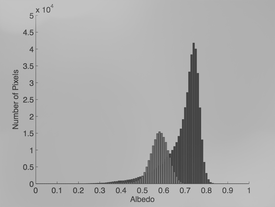
system and study the key governing physical process. Characterizing the ice extent and albedo as a multifractal enabled
us to study the physical processes governing the system, study the variability of melt ponds, examine the annual to decadal
evolution of albedo, and demonstrate the presence of white noise in ice extent on annual to bi-annual timescales. This white
noise characteristic is the principle reason behind unpredictability of sea-ice extent magnitude on these timescales. I then
analyzed the observed Arctic sea ice velocity fields and constructed a periodically forced stochastic model, which explains
the timescales that underlie the observed persistent structure of the velocity field and the forcing that produces it.
I built a simple model of heat and mass transfer in the Fram Strait that revealed some fundamental mechanisms controlling
sea-ice extent in the marginal seas. By analyzing paleoclimate surface air temperature data, I showed the presence
of 1/f noise on multi-decadal timescales and global spatial scales.
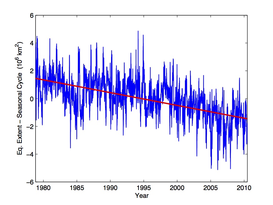
Arctic Equivalent Ice Extent without Seasonal Cycle.
Reproduced from Figure 1 of Agarwal et al. (2012). Equivalent
Ice Extent (EIE) during the satellite era (blue) shown relative to the mean (red) with the seasonal cycle removed.
EIE, which differs from traditional ice extent or ice area, is defined as the total surface area, including land,
north of the zonal-mean ice edge latitude, and thus is proportional to the sine of the ice edge latitude. EIE was
defined by Eisenman (Eisenman, 2010) to deal with the geometric muting of ice area associated with the seasonal bias
of the influence of the Arctic basin land mass boundaries.
Export of Sea Ice in the Fram Strait.
Reproduced from Figure 1 of Agarwal et al. (2017). The warm and salty West
Spitsbergen Current (WSC) flows northwards, which melts the southwards-flowing ice to create a wedge shape, whereas
the relatively cold and fresh East Greenland Current (EGC) flows southwards with the ice and therefore does not show
such a wedge. This figure is a schematic of our simple longitudinal model used to study the dynamics of sea-ice edge in detail.
Spatial Distribution of Shortest Pink Noise Timescale (in years)
Reproduced from Figure 1 of Moon et al. (2018). Spatial distribution of the shortest timescale (in years)
at which pink-noise behavior appears in the GISS data set. This transition takes place on multidecadal timescales nearly every- where. The red color denotes locations that do not show pink- noise characteristics on timescales up to 65 yr (half of the total length of the data set), with the most prominent feature being in the tropical eastern Pacific. White regions show locations where continuous data are absent..
Chaos
The theory of multifractals, chaos, and noise form the backbone of nearly all naturally occurring physical processes. To
examine the interactions between noise and chaos in a well defined setting, we calculated the upper bounds of the stochastic
Lorenz System, and showed that the effect of noise is equivalent to that of chaos.
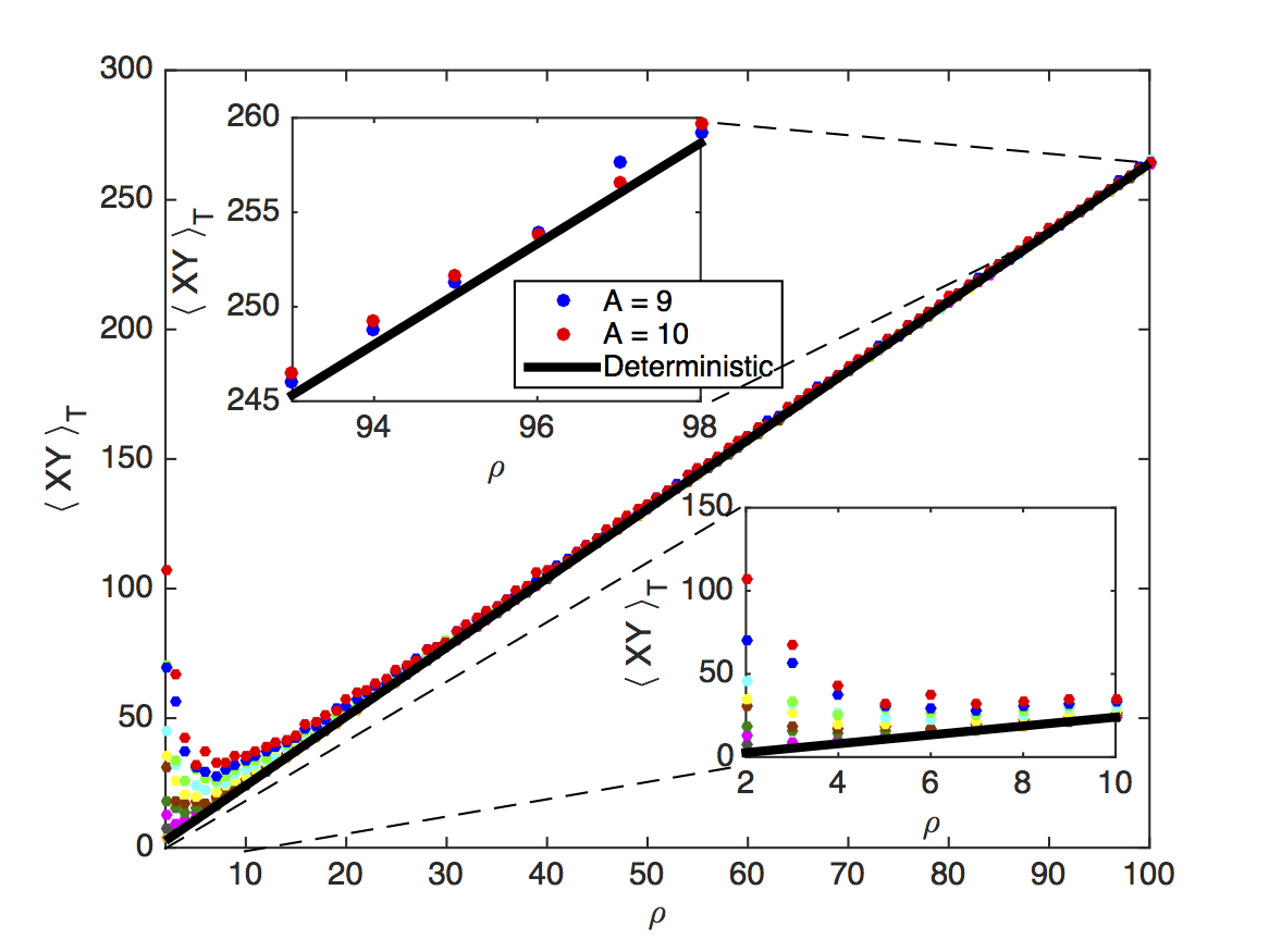
Stochastic Upper Bounds.
Reproduced from Figure 4 of Agarwal et al. (2016). The stochastic upper-bound (SUB)
(circles) as a function of reduced Rayleigh number ρ and noise amplitude A. The solid black line is the
Deterministic Upper Bound. The bottom inset shows that the SUB is a monotonic function of A in the non-chaotic regime
(ρ < ρ
c ). The top inset shows the oscillations of the SUB between noise amplitudes A = 9, 10 in the chaotic regime
(ρ > ρ
c ).
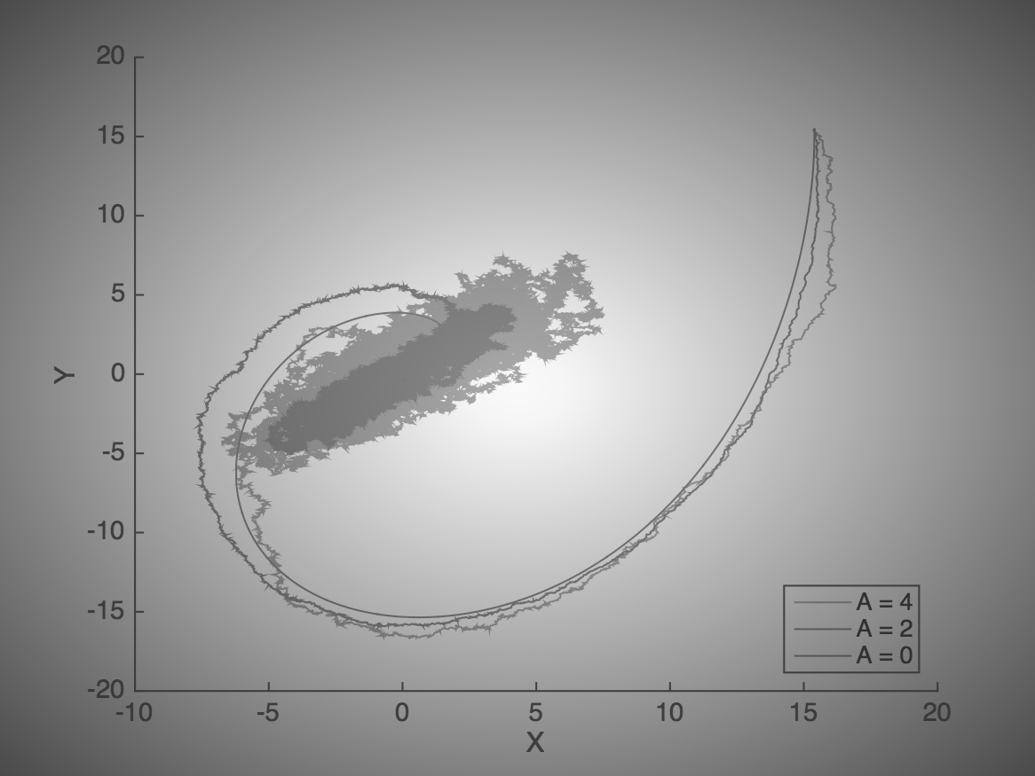
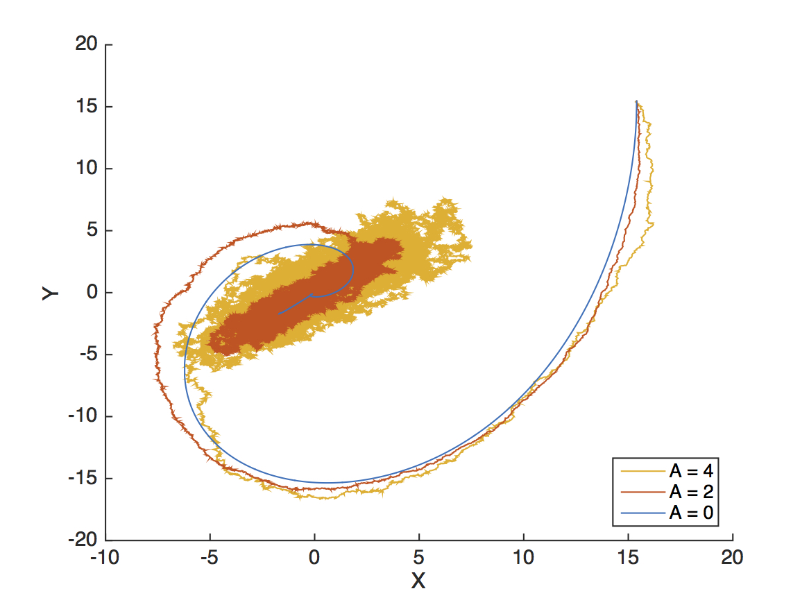
Noise vs. Chaos.
The XY-space of the Lorenz attractor in the non-chaotic regime, showing the
trajectory, as a function of noise amplitude in the system.