Driven IFS and Data Analysis

Traditional and Driven IFS Correlations

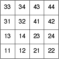
Kalla and Sobhan divided each driven IFS plot up into address length 2 subsquares, and counted the number of data points in each subsquare. Recall the notion of addresses.

Here are the values for these driven IFS, in this format

{{n11,n12,n13,n14}, {n21,n22,n23,n24}, {n31,n32,n33,n34}, {n41,n42,n43,n44}}

where nij denotes the number of points in the square with address ij.

Coca-Cola   {{0,4,0,0},{3,22,44,4},{0,44,109,8},{1,2,9,0}} Kellogg   {{0,0,1,1},{0,1,12,9},{2,16,137,28},{0,6,32,5}} Nokia   {{0,9,3,1},{6,105,44,4},{5,43,21,2},{2,2,3,0}} Motorola   {{0,0,1,0},{0,7,33,5},{1,35,129,16},{0,3,18,2}} Microsoft   {{0,2,1,1},{0,21,38,9},{1,37,100,13},{3,8,12,4}} Chase   {{1,4,1,1},{2,62,55,2},{4,51,58,3},{0,3,3,0}}

In the next section we shall see a way this information can be used to compare the driven IFS pictures.

Retrun to Address correlation.